Page 65 - Textos de Matemática Vol. 36

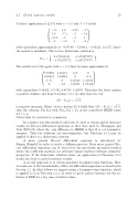
2.5. Global existence results 55 A direct application of (2.47) with a = 1.8 and C = I yields
 −3.6 1.8 −2.65 −1   1.8 −7.2 −1 −3.8 −2.65 −1 −2 1 
−1 −3.8 1 −4
with eigenvalues approximately at −9.87689, −5.59462, −2.95221, 1.62373, hence
the matrix is indefinite. The reverse dichotomic solution is 4.273521323 −1.072471775
Prd := −1.072471772 −2.847173675 .
The matrix in (2.50) again with a = 1.8 then becomes approximately
7.93850 2.28261 1.35 0  2.28261 3.04982 0 −1.8   1.35 0 4.41028 1.26811
0 −1.8 1.26811 1.69434
with eigenvalues 9.18424, 2.63392, 0.06786, 5.20693. Therefore the latter matrix is positive definite and from Corollary 2.5.3 we infer that the ball
√ ||P−Prd||< 1.8
√
is negative invariant. Hence, if for a matrix P0 it holds that ||P0 −Prd|| <
then the solution P(t,P0) with P(t0,P0) = P0 of the considered HRDE exists for t ≤ t0.
Notice that P0 need not be symmetric.
In a similar way this method could also be used to obtain global existence results for Riccati differential equations as they were used by Thompson and Volz [ThVo75] where the only difference to HRDE is that Q is not symmetric anymore. Then the solutions are non-symmetric, but Theorem 2.5.2 may be applied if there is a dichotomic solution.
A more general Riccati differential equation is introduced by Kuiper [Kuip94] in order to study a diffusion process. Even more general Ric- cati differential equations can be treated by the previously presented method where the coefficient matrices are arbitrary square matrices without symmetry properties. If the dichotomic solution exists, an application of Theorem 2.5.2 would also lead to global existence results.
A second approach is to obtain quadratic Lyapunov-type functions. Here we make use of the linearizability of Riccati differential equations as described in Section 2.2. In what follows we suggest using a Lyapunov-type function, which is applied to L in Theorem 2.2.1, in order to prove global existence for the so- lution of RDE for a big class of initial values.
1.8,