Page 150 - Textos de Matemática Vol. 47

140 P. DE ZEA BERMUDEZ, M. A. AMARAL TURKMAN, AND K. F. TURKMAN
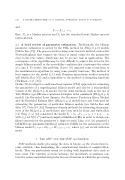
and
Yt = Xt 1 + ✏t.
Here, Xt is a Markov process and Yt has the standard latent Markov process
representation.
2.2. A brief review of parameter estimation. Traditionally, the bilinear parameter estimation is carried by the CML method for BL(p, 0, p, k) models (Subba Rao [35]). The process involves using some iterative method, such as the Newton-Raphson that requires the choice of initial values for the parameters close to the true values, which may not be an easy task in applications. The convergence of the algorithm may be very di cult to achieve due (even for the simple bilinear model) to the invertibility condition that constraints the values of a and b. To reduce this problem, Scotto [33] imposed some restrictions to the maximization algorithm by using some penalty functions. The method of least squares for the model (2.1) with Gaussian innovations works reasonably well (Subba Rao [35]) and is equivalent to the method of estimating functions (Turkman et al. [38]).
Grahn [15] developed a conditional least squares (CLS) approach for estimating the parameters of a superdiagonal bilinear model and also for a standardized version of the BL(p,0,p,1) model. Several other methods, such as the use of Yule-Walker type di↵erence equations for higher order cumulants (BL(p, 0, p, 1) model), the Extended Least Squares, the Recursive Prediction Error Method and the Extended Kalman filter (BL(p, 0, p, 1) model) have also been used for estimating the parameters of particular bilinear models (see Subba Rao and Silva [37], Gabr [19, 20]). Frequency-domain methods for estimating the param- eters of the BL(p, 0, p, 1) model have also been used by Sesay and Subba Rao [34]. Feng et al. [14] considered the model Yt = b✏t 1Yt 2 + ✏t, t = 1,2,...,n, with {✏t} iid N(0, 2) and used empirical likelihood (EL) in order to obtain con- fidence intervals for the parameter b. Quite recently, Ling et al. [26] proposed a GARCH-type maximum likelihood estimator (MLE) for the parameters of the bilinear model Yt = μ + aYt 2 + bYt 2✏t 1 + ✏t, where {✏t} are rvs iid with zero mean.
3. The ABC and the SMC algorithms
SMC methods enable processing the data in blocks, as the observation be- came available, thus diminishing the computational burden of complex likeli- hoods. They are particularly useful for dealing with dependent data, such as time series. The volatility of stock exchange, the movements of airplanes cap- tured by radars and industrial production are situations in which the processing