Page 154 - Textos de Matemática Vol. 47

144 P. DE ZEA BERMUDEZ, M. A. AMARAL TURKMAN, AND K. F. TURKMAN
4. Simulation study: ABC vs. CML
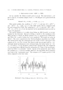
Let us consider the bilinear model given in (2.2). The innovations ✏t are iid rvs N (0, 1). A random sample of size n = 150 (Figure 2) is generated from the model
Model I: Xt = 0.2Xt 1 + 0.4Xt 1✏t 1 + ✏t.
This model satisfies the condition a2 + b2 2 < 1 and also 2(1 + a)b4 4 + 2(1 a)b2 2 (1 a)2(1 + a)  0. The ABC results will be compared with the ones obtained by CML. The conditions a2 + b2 < 1 and 2(1 + a)b4 + 2(1 a)b2 (1 a)2(1 + a)  0 are incorporated in the maximization process just as Scotto [33] proposed.
The initial estimate of a results from fitting an AR(1) model, as recom- mended in the literature. Instead of fitting a model to the residuals of the AR(1) model to obtain an initial estimate for b, as proposed by Subba Rao and Gabr [36], a grid of values for b was considered. The results are given in Table 1. The error considered in the Newton-Raphson algorithm was 0.0001. The models show that the estimation process seems to have converged to the solution (aˆ, ˆb) = (0.1796, 0.3224). The fastest result was attained with b0 = 0.3, although similar performances were obtained using the initial values b0 = 0.1, b0 = 0.2 and b0 = 0.4. It should be referred that, unexpectedly, the estimation of a was much more di cult than the estimation of b. Some of the models pre- sented in Table 1 occasionally “visited” regions of the parametric space where the condition |a| < 1 was not satisfied. However, the algorithm always found its way back to the “stationarity zone”. The estimate of 2 is quite good (⇡ 1.06) when compared to the true value.
0 50 100 150
Observations
Figure 2. Fixed bilinear data sets - Model I (n = 150).
y
−3 −2 −1 0 1 2 3 4