
Page 127 - Textos de Matemática Vol. 47
P. 127
MODELLING TIME SERIES OF COUNTS: AN INAR APPROACH 117
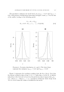
The parameter estimates for model (4.1) are ↵ˆBayes = 0.27 and ˆBayes = 0.89, with posterior distributions represented in Figure 4 and ⌘ˆ = 7 for the size of the outlier, leading to the following model:
Xt = 0.27 Xt 1 + et, (a)
et ⇠ P o(0.89).
(4.2)
Yt = Xt + 7I224,
(b)
0.20 0.25 0.30 0.35
0.70 0.80
0.90 1.00
αλ
Figure 4. Posterior distribution of ↵ and . The dotted lines represent the estimates ↵ˆBayes = 0.27 and ˆBayes = 0.89.
Figure 5 represents the residuals resulting from the fit of (4.2). Note that the largest residual reduces from 6.8 to 3.3, indicating a better fit.PAnfurther indication of the better fit is based on the prediction sum of squares t=2(yt yˆt)2, where yˆt = E(yt|yt 1 = yt 1; parameter estimates) which drops from 317.9 to 264.0 when the outlier is included in the model.
0 5 10 15
Density
Density
0 2 4 6 8 10 12
