Page 20 - Textos de Matemática Vol. 47

10 M. I. GOMES
A comparison of the N and the GJ EI-estimators, respectively given in (4.1) and (4.5), based on small-scale Monte Carlo techniques, led us to the following conclusions:
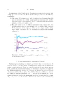
(1) The ‘naive’ GJ estimator of ✓ in (4.5) exhibits for all simulated models and for all values of stable sample paths as functions of k, as illus- trated in Figure 3, for samples of size n = 5000 from ARCH structures with ✓ = 0.1, ✓ = 0.5 and ✓ = 0.9.
(2) For low values of , to which correspond high values of ✓, the
GJ EI-estimator has, at its optimal level, a smaller MSE than the
N EI-estimator, at the expenses of the use of a larger number of top
1.5
values of n. 1.3
1.1
0.9
0.7
0.5 4
5000
0.1 4 5000
-0.1 0
4 -0.3 5000
OS’s. When increases such an advantage no longer holds for small
0.3
0.1 0.1
0.5 0.5
0.9
0.9
! ! 0.9
! ! 0.5
! ! 0.1
1000
2000 3000 4000 5000
k
6000
Figure 3. GJ EI-estimators, in (4.5), for samples of size n = 5000 -0.5
from ARCH processes.
5. A challenge and a tribute to Nazare´
And next goes a challenge to Nazar´e: As I believe that “co-operation is the heart of Science”, we have never co-authored any article, but we have some similar research interests, I hope we can collaborate in the near future in some topic. And I am in particular thinking on the topic I suggested to Nazar´e at her Habilitation Degree: Linking the Choice of the Window in a Kernel Density Estimation with the Choice of the Threshold in Statistics of Extremes. Indeed, the tuning or nuisance parameter h = hn, the size of the window in a kernel density estimation, with n the sample size, needs to be such that hn ! 0 and nhn ! 1, as n ! 1. In statistics of univariate extremes, the crucial tuning
ˆJ
!n (k)